
The vast majority of modern high-class line-following racing robots use a PID controller as the basis for their line-following algorithm. However, for many young robot enthusiasts, the PID controller remains a complex and not well-understood mechanism. Let’s try to understand what a PID controller is and how it works.
What is a “Controller”? #
The concept of a PID controller comes from control theory. This field studies automatic control systems, which we encounter everywhere. Examples include autopilots, torpedo and missile guidance systems, temperature control systems in chemical production, control of absorber rods in nuclear reactors, temperature regulation in air conditioners, and the float valve in a toilet tank. These are all examples of automatic control systems.
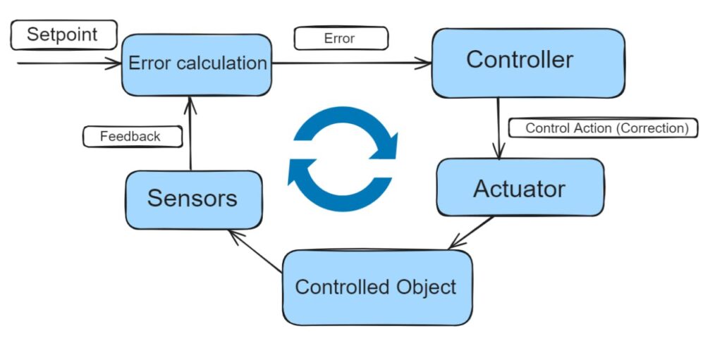
The general diagram of an automatic control system is shown below, and the main concepts of such a system are as follows:
- Controlled Object: This is what the system controls. In the case of a racing robot, it is the robot itself, specifically its position relative to the line.
- Setpoint (Goal, Target Value): This is the condition that the system aims to maintain. For our robot, the goal is to keep it from deviating from the line.
- Error (Control Error): This is the deviation of the current state from the desired state. For us, it’s the robot’s deviation from the line.
- Sensors: These are used to determine the error. For a racing robot, this is usually a “sensor array” — a system of grey sensors (LED/phototransistor pairs).
- Feedback: The signal from the sensors that the system uses to make decisions about corrective actions.
- Controller: The key element of the system. The controller “decides” what actions to take to bring the system back to the target. In a toilet tank, this is a mechanical system, while for a racing robot, it’s the part of the program that implements the PID algorithm.
- Control Action (Correction): These are the actions the system takes to return to the target. For us, it’s adjusting the robot’s motor speeds.
- Actuator: This part of the system implements the control action. In our case, these are the motors.
Calculating the Error #
The first calculation block in this list is calculating the error. An example of how to calculate the error is as follows: assume that each sensor in our sensor array gives an output signal, for example, 200 on a white field and 1000 on a black line. In this case, we can assume that if a sensor shows more than 600, it is over the line. If it shows 600 or less, it is over the white field.
To calculate position error we can use the weighted sum algorithm:
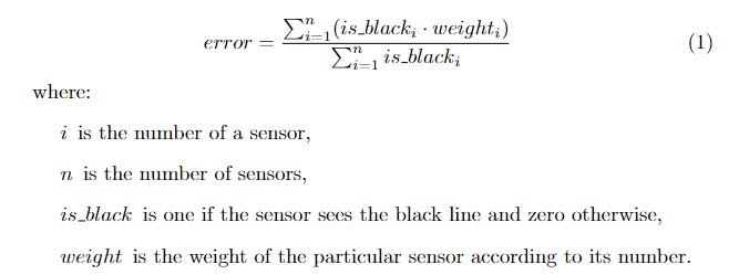
This algorithm for a system of eight line sensors on an Arduino would look something like this:
float bot_position()
{
  float posSum = 0;
  float posMedian = 0;
  float signal[8];

  qtr.read(signal);

  for (int i = 0; i < 8; i++) {
    if (signal[i] > 600)
    {
      posSum += 1;
      posMedian += i * 2;
    }
  }

  if (posSum > 0)
  {
    return posMedian / posSum - 7;
  }
  else
  {
    return 0;
  }
}
Here, signal is an array for storing the signal measurement results from each of the eight sensors, and qtr.read(signal) is a function that fills the array with sensor values. It’s easy to see that this function will return 0 if the line is exactly in the middle of the sensor array and a positive or negative value if the robot deviates to the right or left.
This is a highly simplified error calculation, which usually requires a large number of sensors (8-14 in robot races). Another approach is to calculate the fractional position of the robot on the line, using the fact that our sensor will show intermediate values between 200 and 600 as it moves from the white field to the black line. In some situations, even a robot with an array of three line sensors can perform well using this method.
Feedback #
The second calculation block is feedback. For a simple robot, feedback is typically implemented as follows: the controller calculates a correction value, which is added to the speed of one motor and subtracted from the speed of the other motor.
For example, we set the average motor speed as PWM 150 with 255 being the maximum PWM for our controller. Then, if the calculated control value is 50, we add 50 to the right motor (resulting in PWM 200) and subtract 50 from the left motor (resulting in PWM 100). If the calculated control value is negative, -50, the left motor will move faster instead.
P-Controller #
The “P” in P-controller stands for “proportional.” A P-controller takes the current deviation of the robot from the line and calculates the control action proportional to this deviation.
For example, our error calculation is such that a deviation of the robot by half a sensor from the line gives an error of one unit. So, if the robot deviates by half a sensor, we get an error of 1. If it deviates by one sensor, the error is 2, and if it deviates by two sensors, the error from our bot_position() function will be four.
In this case, we can write the P-controller like this:
int avgSpeed = 150; // Average motor speed
int kP = 10; // Proportional feedback coefficient
int error; // Position error

error = bot_position();
correction = kP * error;

motor1.move(avgSpeed * (1 + correction));
motor2.move(avgSpeed * (1 - correction));
Here, the functions motor1.move() and motor2.move() will control the speed of the left and right motors, from -255 to 255. If the robot deviates by half a sensor, the motor speeds will change: one motor will receive a PWM of 165, and the other 135, causing the robot to move in an arc. Imagine the line under the robot makes a sharp turn, and the robot’s turning radius is still insufficient to get back on the line. In this case, the robot will soon deviate by a full sensor, the error will become two, and the correction will be 20. The motor speeds will then change to 180 and 120, respectively, making the robot try even harder to get back on the line. The sharper the line under the robot turns, the more the robot will deviate, and the greater the speed difference between the motors will be.
How do we tune the kP coefficient? A robot with a low kP is called underdamped. Such a robot cannot turn sharply enough to stay on the line. A robot with a high kP is called overdamped. It starts “jerking” and moving in zigzags, deviating from the line to the right and then to the left. In the video above, you can see that the robot is slightly overdamped — it does not move smoothly but oscillates, sometimes veering the sensor array to the left of the line even while turning left. A well-tuned robot with a P-controller always turns right when the nose is to the left of the line and left when the nose is to the right, as it “seeks the lost line.”
Let’s look at a robot with a significantly overdamped P-controller, and we’ll see that it oscillates constantly:
A P-controller is good for slow robots where inertia does not affect the robot’s movement. Let’s increase the robot’s speed, and we will see that the current kP values are no longer sufficient — the robot starts to deviate. We will need to increase kP to keep the robot on the line. However, this will make the robot overdamped, causing it to move in zigzags. So, it can be both underdamped — not enough kP to stay on the line, and overdamped — moving in a zigzag pattern. The reason for this is inertia. The power and reaction speed of the motors and the wheel traction are not enough for the robot to instantly respond to the controller’s commands. A P-controller is not suitable for controlling robots with inertia, so we need to move on to the next type of controller — the PD-controller.
PD-Controller #
In the video with increased speed, let’s pay attention to which parts of the track are the most difficult for the robot. It is evident that the robot is underdamped on successive turns, i.e., when the robot turns in one direction and then needs to turn in the opposite direction. At this moment, the accumulated inertia comes into play, and the motor power is insufficient to quickly turn the robot in the other direction.
A D-controller (differential controller) works by calculating the change in error over a certain period and then determining the necessary control as the product of this change and a coefficient we denote as kD. We get a PD-controller by adding a D-controller to the existing P-controller.
int prev_error;

void loop(void)
{
  int avgSpeed = 150; // Average motor speed
  int kP = 10; // Proportional feedback coefficient
  int kD = 1; // Differential feedback coefficient
  int error; // Position error

  error = bot_position();
  correction = kP * error + kD * (error - prev_error);
  prev_error = error;

  motor1.move(avgSpeed * (1 + correction));
  motor2.move(avgSpeed * (1 - correction));

  delay(10);
}
We added the variable prev_error, the calculation of the differential correction kD * (error - prev_error), and a delay in the loop — delay(10). As seen from the formula, the D-controller combats rapid changes in error. It helps to counteract inertia and oscillations, making it essential for robots moving at high speeds.
The drawback of the D-controller is that it requires a delay in the control loop. The error value in our case changes infrequently; the robot needs to travel some distance for the error to change. Without the delay, the D-controller will act very briefly, only at the short moment when the robot transitions from one sensor to another. The delay duration should be enough for the error value to change by a couple of sensors. However, what benefits the D-controller harms the P-controller, which loses the ability to react quickly to changes in the robot’s position.
Another drawback of the D-controller is its susceptibility to noise. Random light fluctuations can trigger unexpected responses.
Let’s look at a more professional PD-controller code for our robot:
int avgSpeed = 150; // средняя скорость моторов
int kP = 10; // коэффициент пропорциональной обратной связи
int kD = 5; // коэффициент дифференциальной обратной связи

int correction;
int err;

int err_arr[] = {0, 0, 0, 0, 0, 0, 0, 0, 0, 0};
int err_p = -1;

prevErr = bot_position();

void loop(void)
{
  err = bot_position();
  err_p = (err_p + 1) % 10;
  err_arr[err_p] = err;

  P = err * KP;
  D = (err_arr[err_p] - err_arr[(err_p+11) % 10])*KD;

  correction = P + D;

  motor1.move(avgSpeed*(1+correction));
  motor2.move(avgSpeed*(1-correction));

  delay(2);
}
In this example, the last ten errors are stored in the err_arr array, and the D-controller bases its correction calculation on the difference between the current error value and the error value from 20 milliseconds ago (cycle time of 2ms * 10, where 10 is the number of elements in the array). The D-controller allows for a significant increase in the robot’s speed.
If the differential feedback coefficient is too high, the robot with a PD controller will start to “get angry” or “nervous” — such a robot will exhibit high-frequency oscillations. Unlike an overdamped “P” control, which causes oscillations to the left and right of the desired direction, overdamping with “D” control makes the robot “tremble.”
Let’s reduce the kD coefficient, and we will see that the robot moves much smoother than with the P-controller. Moreover, we can even reduce the kP coefficient, and the robot will still successfully navigate the track. With the PD controller, this robot can move more than twice as fast as with the P-controller.
You can see that the robot now moves as if it has a well-tuned P-controller, even though we know that at this speed, a P-controller alone would not be sufficient. It would need to be highly overdamped, which would be noticeable from its oscillations. The D-controller in our case seems to make the motors more powerful, improves the robot’s balance, and increases the accuracy of the sensor array.
I-Controller #
Notice in the previous video that the robot moves on the “edge sensors” in a turn, significantly deviating from the center of the line. This is a characteristic of the P-controller, which requires the robot to move with some error; without error, there is no correction.
However, there is a simple controller that ensures the robot moves precisely in the center of the line. This is the I-controller (integral controller). Watch the video below — a robot with a well-tuned I-controller moves exactly in the center of the line, even in turns.
It calculates the control action as the product of a coefficient, which I will call kI, and the accumulated error. You can simply sum up all the errors “from the beginning of time.” In our case, I will sum the last ten errors, which we already store in an array.
int avgSpeed = 150; // Average motor speed
int kP = 10; // Proportional feedback coefficient
int kD = 5; // Differential feedback coefficient
int kI = 5; // Integral feedback coefficient

int correction;
int err;

int err_arr[] = {0, 0, 0, 0, 0, 0, 0, 0, 0, 0};
int err_p = -1;

prevErr = bot_position();

void loop(void)
{
  err = bot_position();
  err_p = (err_p + 1) % 10;
  err_arr[err_p] = err;

  P = err * kP;
  D = (err_arr[err_p] - err_arr[(err_p+11) % 10]) * kD;
  int err_sum = 0;
  for (int i = 0; i < 10; i++) err_sum += err_arr[i];
  I = (err_sum / 10) * kI;

  correction = P + I + D;

  motor1.move(avgSpeed * (1 + correction));
  motor2.move(avgSpeed * (1 - correction));

  delay(2);
}
In this code, you see a full PID controller. A robot with a properly tuned PID controller will move along the center of the line. But what happens if the I-controller is over-tuned, with kI set too high? In this case, the I-controller will interfere with the P-controller, and the robot will start to jerk again, as shown in the video below. Usually, the kP coefficient is slightly reduced in a PID controller compared to a PD controller because the integral controller helps the proportional controller.
Tuning a PID Controller #
The usual tuning process for a robot is as follows:
- Tune the P-controller at low speed: Adjust the kP value so that the robot follows the line closely, even in the sharpest turns. During this step, set kD and kI to zero, using only the P-controller.
- Increase the speed and adjust kD: If the robot moved without inertia while tuning the P-controller, you can keep the kP value the same. If the robot had inertia, as is common with fast robots, you will need to lower the kP value. You will see this adjustment when the robot stops deviating significantly from the line, thanks to the help of the D-controller.
- Tune the I-controller: Once the PD-controller is tuned, you can adjust the I value to reduce the robot’s deviations from the line. During this step, the kD and kP values are usually slightly reduced. The I-controller is useful for races where the line may loop. Deviating from a straight path can lead to choosing the wrong direction. For races on tracks without loops, a PD-controller is often used because it generally allows for higher speeds.
What’s Next? #
The algorithms described above are just a small part of what is used in advanced robots. We plan to continue our series of articles on automatic control for racing robots, and I would appreciate any feedback.
Frequently used techniques not covered in this article:
- Line Loss Handling: When the robot loses the line, it makes a sharp turn to find it.
- Non-linear Proportional Controller: A proportional controller depends only on the current error. However, the error calculation (or feedback) can be non-linear. For example, if the line has long, gentle curves plus sharp turns, the controller can be designed to make smooth turns for small errors and sharp turns for significant errors.
- Speed Controller: This article describes a position controller. Often, it’s not the only controller in a racing robot. Speed controllers for the turbine’s rotation speed or the wheels (if there are speed sensors like wheel encoders) are also used. The second most common controller after the position controller is the speed controller. Here, the error is considered the accumulated sum of the error magnitudes. The more the robot deviates, the lower its speed. On a straight path, such a robot will accelerate.
- Fuzzy Controllers: These are an alternative to PID controllers.
- Analog Error Processing from Line Sensors: The signal from the line sensors is converted not into a discrete error (0 or 1) but into a continuous value between 0 and 1.
- Adaptive Controllers: The robot tracks the distance traveled and the line direction (using a direction sensor, IMU) and memorizes the track profile, then adjusts speed, deviation from the line, and PID settings based on the current track section.
- Line Sensor Light Protection and Noise Protection Procedures: Averaging multiple error measurements, for example.
- Automatic Tuning of Controller Parameters Using Gradient Descent.
- Machine Learning and Deep Learning: Modern AI algorithms such as reinforcement learning.
This list is not exhaustive. Hirai Masaaki, a multiple-time All Japan race champion, wrote that he spends 80% of his robot preparation time on movement algorithms and only 20% on construction. This applies to highly advanced robots with custom-made gearboxes, a movable nose section (moving sideways with a servo motor), and custom-made printed circuit boards!


